HomeServerBlog leaf-spine planner
Fabric Bandwidth Calculator
Estimate leaf-spine aggregate capacity, one-way bisection bandwidth, effective usable bandwidth, remote east-west demand, oversubscription, and failure-mode headroom for a home lab or compact server fabric.
1Fabric presets
2Leaf, spine, port, and traffic inputs
Calculation breakdown
Fabric status
3Live fabric design cards
All host ports across all leaves at line rate.
Host edge capacity divided by usable fabric.
Estimated traffic crossing through the spine layer.
Total leaf uplinks to cable into spine switches.
4Fabric design grid
5Bandwidth reference tables
| Fabric shape | Host edge example | Fabric uplink example | Common fit |
|---|---|---|---|
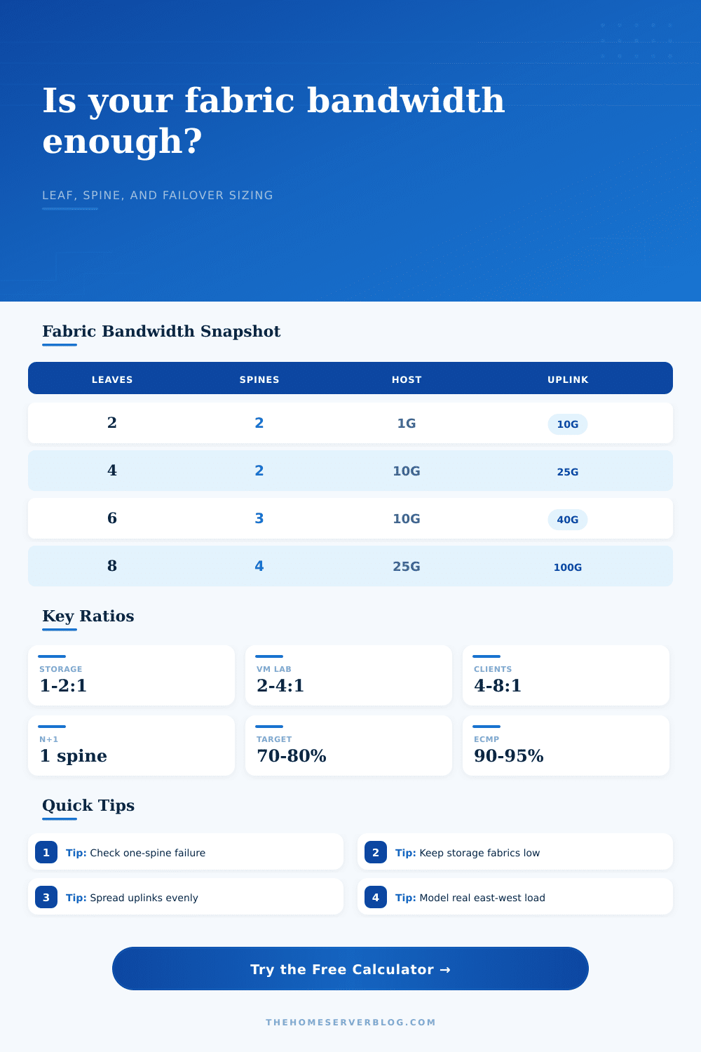
| 2 leaves x 2 spines | 24 x 1G per leaf | 2 x 10G per leaf | Starter server rack, small NAS, router lab, light VM traffic. |
| 4 leaves x 2 spines | 24 x 10G per leaf | 4 x 25G per leaf | Dense home lab, Proxmox cluster, multi-NAS backup paths. |
| 6 leaves x 3 spines | 32 x 10G per leaf | 6 x 40G per leaf | Workshop rack, lab pods, Wi-Fi aggregation, routed VLAN core. |
| 8 leaves x 4 spines | 24 x 25G per leaf | 4 x 100G per leaf | Compact data-center style sandbox with serious east-west demand. |
| Oversubscription ratio | Fabric workload | Risk signal | Planning note |
|---|---|---|---|
| 1:1 to 2:1 | Storage, backup, VM migration, GPU data movement | Host NIC and disk bottlenecks | Useful when east-west traffic is frequent and bursty. |
| 2:1 to 4:1 | General virtualization and mixed home lab services | Busy backup windows | Often a balanced target for 10G or 25G server leaves. |
| 4:1 to 8:1 | Client access, AP aggregation, low-duty workloads | Many simultaneous downloads | Acceptable when telemetry confirms low sustained utilization. |
| 8:1 plus | IoT, cameras, internet-bound client access | Unexpected local replication | Use only with clear traffic assumptions and queue monitoring. |
| Failure model | Capacity rule | What to inspect | Home lab use |
|---|---|---|---|
| One spine down | Capacity scales by remaining spines / total spines | ECMP path loss and spine port symmetry | Best default for routed leaf-spine designs. |
| One uplink per leaf down | Each leaf loses one fabric uplink | Per-leaf oversubscription after link loss | Good for optic, DAC, breakout, or patch failure checks. |
| One leaf isolated | Fabric continues with one fewer leaf | Service placement and storage replica reachability | Useful when one access switch can fail independently. |
| No failure reserve | Normal bisection is reported as failure capacity | Monitoring and manual recovery plan | Bench networks and noncritical lab builds. |
| Uplink generation | Practical bandwidth | Typical media | Design watchpoint |
|---|---|---|---|
| 10G | Good for 1G leaves and small server racks | SFP+ DAC, fiber, 10GBASE-T | Copper heat and limited uplink count on compact switches. |
| 25G | Strong step up for 10G host leaves | SFP28 DAC or fiber | Check NIC, switch, and cable compatibility carefully. |
| 40G | Useful used-market core bandwidth | QSFP+ DAC, SR4, breakout | Breakout lane mapping can complicate even leaf spread. |
| 100G | Compact high-density lab fabric | QSFP28 DAC, SR4, LR4 | Optics, airflow, and switch power become part of the design. |
| 200G / 400G | Advanced sandbox or lab validation | QSFP56, QSFP-DD, OSFP | Endpoint capability may be the real limiting factor. |
6Fabric bandwidth tips
Sooner or later you’ll be at this stage with your home lab: Your rack has turned from a group of shiny boxes into a knotted mass of cables. You’ve added a new storage array, or perhaps another server. The network grind to a halt. Chances are good that it’s bandwidth starvation, not some kind of switch failure. Traffic volume exceed the pipes’ capacity.
How do you get data around? What if something breaks? That’s why it matters how you size your fabric. These is the models from the calculator that combine bisection bandwidth and capacity. The important part is bisection bandwidth.
How to Plan Your Home Lab Network
That’s the bandwidth between two server talking to each other when you cut the fabric in half. Every server on one side of the fabric talk to every other server on the opposite side of the fabric.
How does this relate to oversubscription? Oversubscription means you have more bandwidth coming into your hosts (capacity) than you do going between them (bisection bandwidth). There’s nothing wrong with being oversubscribed, it just makes your system cheaper. You want to understand how oversubscribed you can be before VMs start timing out during a migration, or a backup fails.
Consider what traffic is being moved. Is the storage fabric using NFS or iSCSI? This is a latency-sensitive protocol, so you want to keep oversubscription low, maybe one to two to one. Are the VMs mostly idle? Use a higher ratio, maybe four to eight to one. Oversubscription is where you set a target, which the tool does for you. Then it tells you whether your hardware will support that. It doesn’t make you guess at whether twenty-four ten gigabit host ports can handles twenty-five gigabit uplinks.
You must design for failure scenarios, because most designs fall apart when they fail. Lots of folks design for the happy path; where everything works and all switches are up and running. That’s unrealistic. Model a failure. When a spine switch fails, how much does the rest of the spine have left to be able to handle the load of all those leaves? Simulate what happens with a one-spine failure. You’ll probably notice the usable bandwidth is greatly reduced. If that falls below your critical workload needs, you’re going to have a problem. That’s why n plus one redundancy matter. It keeps the lab running even if there is a failure and the workload shift.
People get surprised by how much traffic is east-west. Most traffic in a home lab or even a moddern data center doesn’t leave the local network. Containers talk to their databases, and servers talks to other servers. That traffic go through the spine layer. Underestimating the percent of east-west traffic will lead you to underestimate the amount of load your spines must handle.
Ask yourself what percent of your traffic is east-west. For example, if you have a Proxmox cluster doing lots of storage replication/live migration, then that’s a higher number. If you’re mostly serving files to a handful of Windows PCs, then that’s lower.
The symmetry also works here. Each leaf need an equal number of uplinks to an equal number of spines. That way Equal-Cost Multi-Path routing can do its job and spread things around evenly. You don’t want one leaf with two uplinks and another with four because then you’ll bottleneck your setup. Leaf and spine counts is interlinked as the tool’s reference table shows. It can be a good guide for keeping away from silly topologies that won’t work in real life.
Don’t overlook the physical layer either. Fewer wires equals fewer points of failure, less heat, etc. More speed on the uplink also means fewer links. For example, a switch with ten gigabit uplinks can easily be upgraded to twenty-five gigabits without adding more links. That is generaly better than having to add more links. Make sure you have the right DACs for the job, and make sure your switches support it.
Hardware matter; it makes all the difference in how well the math works out. You should of considered this earlier. The strength of a fabric is defined by its weakest link in a failure. Use the numbers to guide your buying decisions and plan for the worst. Your network should feel invisible, no one ever hits their limit.