HomeServerBlog optical planning worksheet
Fiber Bandwidth Distance Product Calculator
Estimate whether OM1, OM2, OM3, OM4, OM5, OS1, or OS2 fiber has enough bandwidth-distance product for a target link distance, aggregate data rate, wavelength, launch style, channels, connector allowance, dispersion penalty, and engineering margin.
1OM and OS fiber presets
2Bandwidth, distance, and optical inputs
Calculation breakdown
Pass margin view
3Multimode and single-mode grid
Aggregate data rate divided by lane, wavelength, or channel count.
Estimated aggregate rate at the entered distance after penalties.
Internal BDP math uses kilometers because modal bandwidth is MHz-km.
Launch, loss, dispersion, and reserve margin converted to an effective product.
4Fiber grade reference tables
Multimode modal bandwidth planning values
| Fiber grade | Core | 850 nm OFL / EMB | 1300 nm OFL | Typical planning note |
|---|---|---|---|---|
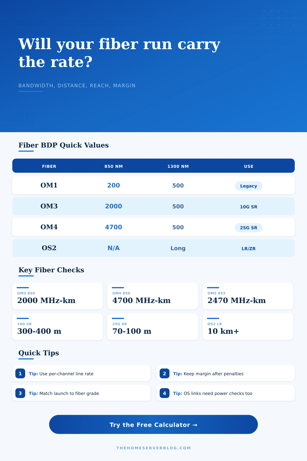
| OM1 | 62.5/125 | 200 MHz-km OFL | 500 MHz-km | Legacy LED and 1000BASE-SX closets; avoid for new high-rate trunks. |
| OM2 | 50/125 | 500 MHz-km OFL | 500 MHz-km | Works for many 1G runs and short 10G lab links with conservative margins. |
| OM3 | 50/125 | 2000 MHz-km EMB | 500 MHz-km | Common minimum for 10GBASE-SR around 300 m under standard assumptions. |
| OM4 | 50/125 | 4700 MHz-km EMB | 500 MHz-km | Preferred for longer 10G SR and higher-rate SR4 building backbones. |
| OM5 | 50/125 | 4700 MHz-km EMB | 500 MHz-km | Wideband MMF; 953 nm support matters for SWDM optics. |
Single-mode OS planning context
| Fiber grade | Mode type | Common wavelengths | BDP handling | Primary practical limit |
|---|---|---|---|---|
| OS1 | Single-mode indoor | 1310 / 1550 nm | Use high equivalent product | Transceiver budget, connectors, and indoor cable attenuation. |
| OS2 | Single-mode outdoor / loose tube | 1310 / 1550 nm | Use high equivalent product | Optic class, chromatic dispersion, splice count, and power margin. |
| G.652.D | Low-water-peak SMF | 1260-1625 nm | Not modal-limited | Power budget and dispersion tolerance at higher rates. |
| Bend SMF | G.657 family | 1310 / 1550 nm | Not modal-limited | Macrobend loss, connector condition, and module specification. |
Common Ethernet reach checkpoints
| Standard family | Common fiber | Nominal wavelength | Common reach | What this calculator checks |
|---|---|---|---|---|
| 1000BASE-SX | OM1 to OM4 | 850 nm | 220-550 m | Whether modal bandwidth is plausible after launch and margin. |
| 10GBASE-SR | OM3 / OM4 | 850 nm | 300-400 m | Whether product headroom remains for the chosen distance and rate. |
| 25GBASE-SR | OM3 / OM4 | 850 nm | 70-100 m | Whether high per-lane rate consumes the available product too quickly. |
| 40G / 100G SR4 | OM3 / OM4 | 850 nm | 70-150 m | Whether lane count lowers per-channel demand enough for the run. |
| 10G / 25G LR | OS1 / OS2 | 1310 nm | 10 km | Equivalent BDP is usually not limiting; check power budget separately. |
| 100G LR4 / CWDM4 | OS2 | 1310 nm band | 2-10 km | Per-wavelength rate, dispersion allowance, and optical margin context. |
Launch and penalty assumptions
| Input | Typical setting | Calculator effect | Use when | Planning caution |
|---|---|---|---|---|
| Overfilled LED launch | 0.75 factor | Reduces usable product | Legacy LED or unknown multimode launch | Conservative for older OM1 and OM2 links. |
| VCSEL laser launch | 1.00 factor | Uses listed EMB directly | 10GBASE-SR, 25GBASE-SR, SR4 modules | Fiber must be laser optimized for optimistic values. |
| Mode conditioning | 0.92 factor | Holds back some product | LX over multimode or mixed plant | Follow the optic vendor patch-cord guidance. |
| Connector loss | dB input | Adds optical stress factor | Patch panels, couplers, dirty or unknown faces | Loss is mainly a power-budget issue, not pure modal bandwidth. |
| Dispersion penalty | dB input | Reduces effective reach | High rates, older fiber, long OS spans | Use module specs when available. |
5Practical BDP tips
Pulling the cable tray cover you see a yellow fiber bundle running from the rack to the patch panel. It’s labeled OM3. It is also labeled as being installed in 2014.
Your new switch want to run 25G SR optics. But your network diagram states that the fiber has been rated for 10G with 300 meters. So do you just plug it in and hope?
What Is the Bandwidth Distance Product?
You seldom see reliable infrastructure being built like this. It isn’t about whether the light turns green. It is about whether the modal bandwidth can handle the data rate over the specified distance. It must does this without turning signal into digital soup.
What’s the answer? That’s the bandwidth distance product. It multiplies the distance of a link by the bandwidth capacity of fiber used.
For multimode fiber, it has something called modal dispersion. What does that mean? Light travels down the fiber as multiple rays. These rays will follow different paths to the other end. Some bounce around the wall. Some go straight through. They hits the other end at different times.
If your data pulses are short enough, the trailing edge of one bit smears into the leading edge of next. The trailing edge of one pulse bleeds over into the leading edge of the next. Errors result.
Plug your rate and your fiber grade into the calculator above, and it’ll do the math for you. No more guesswork on conversions and coefficients.
Engineers think about attenuation. How much power will be lost across that distance? That’s important when you have a single-mode link that span several kilometers.
In the case of short, multimode data-center runs, attenuation isn’t usually the problem. Instead, the problem is dispersion. There’s enough light to run up the fiber, but there aren’t enough edges.
If you pick OM3 or OM4 in the tool, what you’re picking is an effective modal bandwidth rating, which means they offers 2000 and 4700 MHz-km, respectively. That figure isn’t a speed; it’s the ability of the fiber to resolve high-frequency signals across one kilometer.
Launch conditions matter. Maybe your fiber is perfect. Maybe your connectors are cheap. In restricted mode, launching excites less of the fiber core. It makes it look better on quick testing. It is misleading.
In the real world there are multiple patch panels. There are splices. There’s wear. With this tool you can account for dispersion penalties and connector loss to make it more realistic. Ignore that stuff, and you are designing for a lab environment.
Your production stuff will be livig in a hot and dusty rack.
Then we have single-mode fiber, which is a different beast altogether. It has a tiny core. It has almost no modal dispersion. There, your constraints are power budget and chromatic dispersion. The bandwidth distance product does not constrains single-mode links.
That’s why the calculator handles single mode links differently. Instead of bandwidth distance product, what matters is the transceiver power budget. There must be enough light to reach receiver. Not enough light, it’s noise. Too much light, you saturate the detector.
We tend to think of these fiber specs as fixed. But they’re not. Running 2000 MHz-km of 850 nm rated OM3 fiber doesn’t mean it’s a magic bullet. If you double the data rate, you get half the usable distance. (OK, roughly.) It’s an inverse relationship. To run 100 meters versus 50 means twice the bandwidth.
Why does this matter? Well, because OM3 to OM4 upgrades buy you more then marketing. They buy you margin. This lets you run higher rates across the same physical plant.
Now, double-check the reach estimate. It is trouble if that number is negative. Shorten your run. Upgrade your fiber. Change optic types. But don’t try negotiating with physics.
25G over OM3 fiber at 100 meters? Pushing it. In some labs, it’s fine. In others, it’s not. Connector quality and/or launch condition are usually what make the difference.
Margin is never optional when planning. You know dirty connectors and old cables happen. You know what? A 20 percent reserve covers the unknowns.
Margin for the unknown is your 20 percent. You need margin for the quick replacement of a patch cord. It is for that unspotted bend. It is for whatever goes wrong.
And you can see where that margin went in the results breakdown. Notice how much usable product there was vs how much required product. That’s how close or far off you were. And if it was required more than you had usable, you’re going to get some errors.
It’s fast. It’s reliable. It’s durable. But it ain’t endless. The bandwidth distance product is what keeps you from making an expensive mistake. It’s what makes a blind plug-in a planned design. It lets you know your limits before pulling the cable.