Fiber Chromatic Dispersion Calculator
Estimate accumulated chromatic dispersion, residual pulse spread, usable reach, and timing margin for single-mode optical links, CWDM/DWDM waves, and lab transceiver trials.
Calculation breakdown
Link risk meter
G.652 SMF
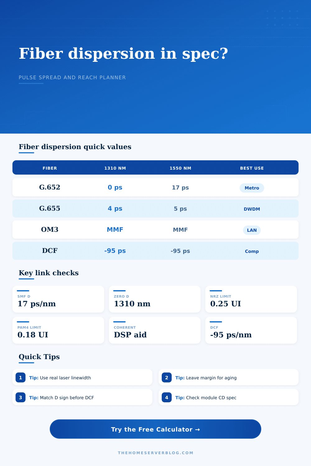
17 ps/nm-km1550 nm typicalCommon outside plant and campus single-mode fiber. Dispersion is low near 1310 nm and much higher in the C-band.
G.657 SMF
16.8 ps/nm-kmbend insensitiveOften behaves like standard SMF for dispersion planning while improving bend performance in panels and building entries.
G.655 NZDSF
4.5 ps/nm-kmDWDM friendlyNon-zero dispersion shifted fiber keeps C-band dispersion lower while avoiding the strongest nonlinear mixing risks.
DCF module
-95 ps/nm-kmcompensationUsed to cancel accumulated positive dispersion, but it usually adds insertion loss and must match the channel plan.
| Fiber / medium | Typical D | Window | Planning note |
|---|---|---|---|
| G.652 standard SMF | 0 to 17 | 1310 / 1550 nm | Near zero at 1310 nm; C-band links need a CD check as length rises. |
| G.657 bend-insensitive SMF | 16 to 18 | 1550 nm | Use standard SMF values unless the cable datasheet says otherwise. |
| G.655 NZDSF | 3 to 6 | 1550 nm | Useful for dense wavelength systems with lower uncompensated CD. |
| DCF / DCM | negative | C-band | Applied as ps/nm compensation, not just fiber length substitution. |
| Transmitter | Spectral width | Direct impact | Use case |
|---|---|---|---|
| DFB laser | 0.05 to 0.15 nm | Low pulse spread | 10G, 25G, 100G lanes |
| EML source | 0.02 to 0.10 nm | Lower chirp | Longer direct-detect links |
| FP laser | 1 to 3 nm | High spread | Shorter legacy links |
| Coherent laser | Very narrow | DSP dominated | 100G to 800G transport |
| Modulation | Bits / symbol | Default limit | Planning behavior |
|---|---|---|---|
| NRZ / OOK | 1 | 0.25 UI | Simple intensity links often use conservative pulse-spread limits. |
| PAM4 | 2 | 0.18 UI | Smaller eye openings make residual dispersion less forgiving. |
| Coherent QPSK | 2 | 0.60 UI | DSP can tolerate far more CD than direct detection. |
| Coherent 16QAM | 4 | 0.45 UI | Higher spectral efficiency usually needs stronger OSNR and margin. |
| Scenario | Length | Watch item | Typical action |
|---|---|---|---|
| Campus LR | 2 to 10 km | Usually mild CD | Confirm optic reach and connector loss. |
| Metro ER | 25 to 40 km | C-band CD rises | Check module CD tolerance before turn-up. |
| ZR / DWDM | 70 km plus | Residual CD | Use DCM, coherent DSP, or lower D fiber. |
| Lab spool | Variable | Wavelength mix | Use the actual source wavelength and linewidth. |
Planning result only. Validate against the optic vendor dispersion limit, receiver sensitivity, optical power budget, connector loss, OSNR, polarization effects, nonlinear penalties, splice records, and field measurements before changing a production fiber link.
Here’s how it works: Glass lets light travel through at varying rates based off color. And since each optical signal you fire down a fiber optic cable consists of a bunch of slightly different wavelengths, they all has to travel as bundle. The slower colors lag while the faster ones pull ahead, causing the whole bundle to spread out as it travels along. This phenomenon is called chromatic dispersion which blurs crisp digital pulses into shapeless blobs that look more like analog noise then clear ones and zeroes. When those blobs gets too close together, they cause errors in your receiver, resulting in bit loss.
After selecting the fiber type, enter in the source specifications and length of your route. The calculator does math for you. You don’t have to dig through a heavy PDF trying to find correct coefficients.
How Dispersion Works and How to Fix It
It’s not just enough to think that all single-mode fiber is identical. G.652 standard fiber differs from G.655 non-zero dispersion-shifted fiber. Standard fiber has almost no dispersion around 1310 nanometers. However, it then shoots up dramatically to roughly 17 picoseconds per nanometer per kilometer at 1550 nanometers.
Why does this matter? Because that’s precisely where most long haul traffic sits, in the C-band. And it’s right there in the C-band that dispersion become the problem.
You’ll never get past knowing what kind of glass you’re working with until you can consider distance. Next up are transmitter specs. Planning fail if you ignore the transmitter. Lasers aren’t perfect point sources, so every laser has a spectral width (how many colors does it realy emit?). A cheap Fabry-Perot laser can be spread across a couple of nanometers. A decent distributed feedback laser’s less than 0.1 nanometer. That make a big difference to pulse broadening.
Pump ten gigabits per second through forty kilometers of ordinary fiber using a wide-spectrum laser, and you’re probably pushing your tolerance limit. Narrowing down that source width gets you more reach then shortening the fiber ever would.
That’s where the modulation format comes into the picture. The rules change depending on what modulation type is used. Eye diagrams of NRZ signals are forgiving: the eye remains wide open. With PAM4 signals, the eye is tight. And those voltage margins between levels is smaller. That’s how reality shows up on the calculator. When you switch to higher-order modulation, there’s less budget to play with. There is less room for error in signal shape. A small tradeoff, yes, but one that determines whether your link drops packets during peak traffic or survives a hot summer day.
And then there’s compensation. To compensate for the buildup you add dispersion compensating fiber. But there are penalties. DCF has high attenuation. So, you are swapping out one problem (dispersion) for another (power budget). With coherent optics, they approaches it differently. It shifts the penalty to the chip and the digital signal processing inside. With coherent optics, you can accept a lot more residual dispersion than direct-detect receivers can.
There are still hard limits. With this tool, you can subtract compensation from total accumulation and figure out how much is left over.
The engineering margin field is also important, and it is not to be ignored. Networks grow old. Fiber degrades a little bit. Splices loses their performance a little. Dirt accumulates on connectors. The temperature changes, and with that the fiber properties does as well. And those shifts move the zero-dispersion wavelength by just a little bit. Twenty percent margin isn’t livig on the edge of disaster. When the world moves around, your link will still be up.
Dispersion is a combination of fiber type, source width, and length. Most folks believe it’s a simple distance issue. It actualy isn’t. Dispersion is really a product of distance, source width, and fiber type. If one of those things is within your control (fiber path or source), you may not need to throw money at costly compensation hardware. The calculator helps you identify the bottleneck. Run low on fiber? Check your spectral width first. Reaching the end of the road? Check your modulation tolerance next time. The connection between these parameters makes sense of an otherwise confusing spec sheet, and transforms what could of been a difficult design decision into something that becomes achievable by thoughtful input selection.
Light will always spread in glass. But with some guidance, you’ll be able to maintain pulse shape sufficiently for reception.