HomeServerBlog optical transport worksheet
Optical Amplifier Gain Calculator
Plan EDFA, Raman-assisted, and SOA amplification by comparing gain, total and per-channel output power, span recovery, VOA trim, estimated OSNR, and saturation headroom before patching a WDM or lab fiber span.
1EDFA and SOA presets
2Amplifier, channel, and span inputs
Calculation breakdown
Amplifier status
3Live amplifier indicators
Input power implied by channel count and per-channel level.
Total output after the entered downstream span loss.
Gain needed to hit target output after VOA attenuation.
Estimated gain reduction as output nears saturation.
4Amplifier type comparison grid
5Amplifier planning tables
Typical EDFA and SOA operating ranges
| Amplifier family | Typical gain | Noise figure | Saturation output | Practical note |
|---|---|---|---|---|
| EDFA booster | 15 to 25 dB | 5 to 7 dB | 17 to 24 dBm | Works well after muxes when per-channel launch is capped. |
| EDFA preamp | 20 to 35 dB | 4.5 to 6 dB | 10 to 18 dBm | Favors low input powers and receiver-side OSNR recovery. |
| Inline EDFA | 17 to 25 dB | 5 to 6.5 dB | 18 to 23 dBm | Usually set close to span loss plus add-drop loss. |
| SOA | 10 to 20 dB | 6 to 9 dB | 8 to 16 dBm | Compact, fast, and useful for labs, but nonlinear earlier. |
| Raman hybrid | 10 to 18 dB | 2.5 to 5 dB | Span dependent | Improves effective noise figure on long single-mode spans. |
Per-channel output targets by channel count
| Channels | -3 dBm/ch total | 0 dBm/ch total | +2 dBm/ch total | Use case |
|---|---|---|---|---|
| 4 | 3.0 dBm | 6.0 dBm | 8.0 dBm | Small CWDM or lab mux |
| 8 | 6.0 dBm | 9.0 dBm | 11.0 dBm | Compact metro shelf |
| 16 | 9.0 dBm | 12.0 dBm | 14.0 dBm | Dense lab or access ring |
| 40 | 13.0 dBm | 16.0 dBm | 18.0 dBm | DWDM line system |
| 80 | 16.0 dBm | 19.0 dBm | 21.0 dBm | High-count line amplifier |
OSNR planning bands in 0.1 nm bandwidth
| Estimated OSNR | Status | Typical modulation fit | Next action | Watch item |
|---|---|---|---|---|
| 35 dB or higher | Comfortable | Most direct-detect lab links | Check receiver overload and launch limits. | Do not overdrive short spans. |
| 28 to 35 dB | Good | 10G and many 25G links | Reserve margin for aging and patch changes. | Connector contamination. |
| 22 to 28 dB | Usable | Conservative direct-detect plans | Reduce loss or lower noise figure if possible. | Cascaded amplifier noise. |
| 18 to 22 dB | Tight | Lab-only unless optics permit it | Measure with an OSA before production use. | FEC margin and BER. |
| Below 18 dB | Risky | Usually marginal | Rework gain, span loss, or amplifier type. | ASE noise buildup. |
Gain and saturation troubleshooting table
| Symptom | Likely cause | Calculator clue | Adjustment | Risk |
|---|---|---|---|---|
| Output misses target | Insufficient gain | Required gain exceeds set gain | Raise gain or reduce pre-amp loss | OSNR may fall if cascading amps |
| Gain compresses | Output near saturation | Headroom below 3 dB | Lower channel power or split bands | Nonlinear distortion and tilt |
| OSNR too low | High noise figure or low input | OSNR margin below target | Use lower NF, cleaner input, or Raman aid | BER and FEC stress |
| Receiver overload | Too much output after span | After-span power too high | Add VOA or lower gain | Optic alarms and errors |
| Uneven channels | Gain tilt or mux mismatch | Total output looks fine only | Measure each wavelength separately | Weak edge channels |
6Practical amplifier tips
First of all: Light gets weaker as it passes down the fiber. That’s how physics works, and there’s nothing you can do about it. Engineering isn’t about preventing loss; its about calculating exactly how much power you need to inject to make up for it.
Too little power and signal vanishes in the noise. Too much power and the distortions gets so excited that they destroys the data just as surely as if the fiber were silent. This balancing act is what optical amplifiers are for, and no one knows how to set them except by careful calculation, not guesswork.
How to Balance Power and Noise in Fiber Optics
A common mistake among many designers is to immediately focus on the gain number and think that greater is obviousely better. However, more gain won’t help you if the amp is already reaching maximum output power. At that point, the amp is “saturated”, meaning it has compressed its output (reducing gain) and increased noise.
By running the calculator above, you can track both gain and saturation headroom so you’ll know if your selected output power is dangerously near the compression point…or comfortabley far enough below it. Leave yourself a few dB of wiggle room and you’re not just building a system for stability but one that holds steady from channel-to-channel.
There’s a lot of noise with this kind of design. Each amplifier adds some background static to your signal. This is called amplified spontaneous emission. That’s called the noise figure. Noise figure represents tradeoff between the amount of amplification you get vs. How much additional static you’re taking on your signal. With a narrow optical signal-to-noise ratio, a high noise figure will eat up your margin fast.
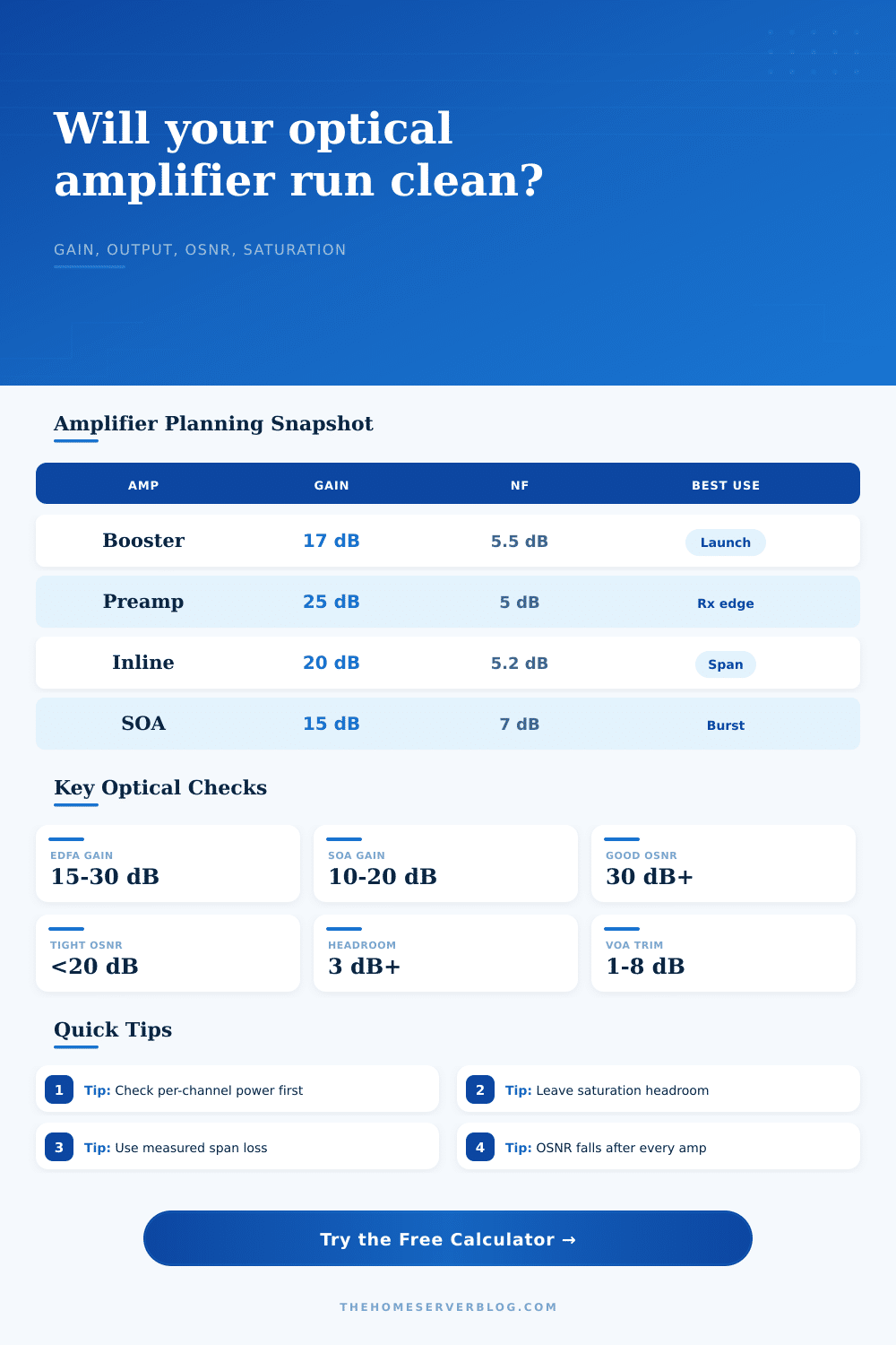
Based off the parameters you enter, the calculator computes your final OSNR and gives you a reality check ahead of time. For most moddern protocols, it should come out at 30 or better. Less than 20 decibels is cause for concern. You may want a different topology or a less noisy device.
The numbers aren’t everything; selecting the right amplifier also make a difference. Most of the time erbium doped fiber amplifiers (EDFA) are used, but the location where it’s placed determines how well it perform.
An EDFA located in front of receiver is called a preamplifier and rescues a weak signal. This one must have lowest noise figure to preserve whatever signal may remain. An EDFA located behind the multiplexor launches the power out into the span and is therefore called a booster amplifier. A booster amp needs high output capacity but can tolerates a slightly higher noise figure.
These differences are shown in the preset selections in the tool which loads realistic parameters for each function. Don’t try to do a preamp job with a booster configuration. That noise penalty will kill you.
This balance is where variable optical attenuators come into play. These act as passive losses and also work as active trimmers that let you decreases gain until you reach a specific target. When your amplifier provide more than necessary, the VOA pulls it back without adjusting your core gain stage. This loss gets factored into the headroom and final output on the calculator. This will keep signal level reaching your receiver in its linear operating range.
Driving your receiver over will create as many errors as driving it below. In real world installs, things don’t stay still. Connectors degrade, fiber bends and temperatures affects loss profiles. Over time, your carefully calculated numbers will shift.
A maintenance strategy of leaving yourself headroom allows you some breathing room to troubleshoot. Designing with margin prevents little changes from becoming crisis situations. If you would of designed right on the edge, then any little thing becomes an issue.
The interface has reference tables that describe typical operating range so you have something to use as a guide. Adjust for your unique span loss and number of channels, but let them be your starting point.
The math isn’t complicated, but consequences for long term reliability are significant. Optical transport is all about managing expectations. You cannot eliminate noise or loss, but with sufficient planning, you can manage them sufficiently to keep them in check.
Let the tool do the arithmetic, so that you can concentrate on the architecture. Verify your OSNR margin and make sure you don’t oversaturate your channels. Patch the fiber when you’re sure you still have saturation headroom left. It prevents spending hours troubleshooting later. The light fades but doesn’t need to dissapears entirely.