HomeServerBlog RF link planner
SNR to Throughput Shannon Calculator
Convert receiver SNR into theoretical Shannon capacity, capped modulation throughput, usable goodput, and target margin for Wi-Fi, LoRa, fixed wireless, cellular, satellite, coax, and lab RF links.
1RF and link presets
2Shannon and implementation inputs
Formula breakdown
Link verdict
3Technology comparison grid
4Live planning cards
SNR after margin, interference, and noise bandwidth factor.
Modulation cap multiplied by FEC rate.
Which ceiling controls the final payload estimate.
Approximate planned SNR needed for the target before reserves.
5Shannon and modulation tables
| SNR dB | Linear SNR | Shannon bps/Hz | Practical note |
|---|---|---|---|
| -10 dB | 0.10x | 0.14 | Useful only with very robust coding, spreading, or low payload expectations. |
| 0 dB | 1.00x | 1.00 | Signal and noise power are equal; margin is scarce. |
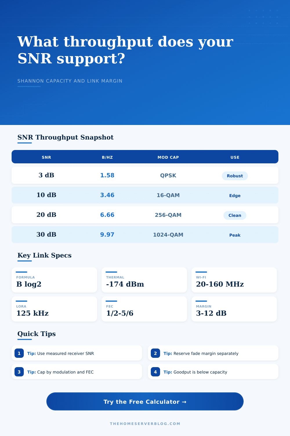
| 3 dB | 2.00x | 1.58 | Low-order modulation and strong FEC are realistic. |
| 10 dB | 10.0x | 3.46 | Edge Wi-Fi, telemetry, or modest QAM planning range. |
| 20 dB | 100x | 6.66 | Clean link with room for 64-QAM or 256-QAM style rates. |
| 30 dB | 1000x | 9.97 | Excellent RF path where hardware and modulation often cap throughput. |
| 40 dB | 10000x | 13.29 | Lab-grade SNR; oscillator, ADC, and front-end limits become visible. |
| Modulation | Raw cap | With 3/4 FEC | Typical SNR planning range |
|---|---|---|---|
| BPSK | 1 b/Hz | 0.75 b/Hz | Very weak or long-range links around 0 to 5 dB. |
| QPSK | 2 b/Hz | 1.5 b/Hz | Robust service from roughly 4 to 10 dB. |
| 16-QAM | 4 b/Hz | 3 b/Hz | Moderate links around 10 to 16 dB. |
| 64-QAM | 6 b/Hz | 4.5 b/Hz | Good links around 16 to 22 dB. |
| 256-QAM | 8 b/Hz | 6 b/Hz | Clean Wi-Fi and fixed links around 22 to 28 dB. |
| 1024-QAM | 10 b/Hz | 7.5 b/Hz | Excellent near-AP or short RF paths around 28 dB and above. |
| 4096-QAM | 12 b/Hz | 9 b/Hz | Peak modern WLAN/lab links with very clean SNR. |
| Bandwidth | Thermal noise | With 5 dB NF | Common link |
|---|---|---|---|
| 12.5 kHz | -133.0 dBm | -128.0 dBm | Narrowband voice, paging, or packet telemetry. |
| 125 kHz | -123.0 dBm | -118.0 dBm | LoRa-style ISM sensor channels. |
| 1 MHz | -114.0 dBm | -109.0 dBm | Lab IF, SDR capture, or narrow data channel. |
| 10 MHz | -104.0 dBm | -99.0 dBm | LTE-style or fixed wireless slice. |
| 20 MHz | -101.0 dBm | -96.0 dBm | Common Wi-Fi channel baseline. |
| 80 MHz | -95.0 dBm | -90.0 dBm | Wide Wi-Fi or high-rate RF link. |
| 160 MHz | -92.0 dBm | -87.0 dBm | Very wide Wi-Fi, 6 GHz, or lab path. |
| Technology | Typical bandwidth | Usable efficiency | What usually limits goodput |
|---|---|---|---|
| Wi-Fi client link | 20 to 160 MHz | 35-70% | Contention, retries, guard interval, MCS changes, and airtime share. |
| LoRa or long-range IoT | 7.8 to 500 kHz | 5-25% | Spreading, coding, duty cycle, preambles, and sensitivity target. |
| Fixed wireless PtP | 10 to 80 MHz | 55-82% | Fade margin, Fresnel clearance, channel width, and chosen MCS. |
| Cellular sector | 5 to 100 MHz | 30-65% | Scheduler share, user load, MIMO rank, CQI, and interference. |
| Satellite / DVB | 5 to 72 MHz | 45-75% | Rain fade, Eb/N0 requirement, MODCOD choice, and roll-off. |
| Coax or lab RF | 1 to 1000 MHz | 70-92% | ADC ENOB, phase noise, filters, amplifier linearity, and modulation cap. |
6SNR throughput tips
Having a full Wi-Fi signal doesn’t mean web pages load fast. The data arrive with high volume. That’s called signal strength. Signal strength tell you how loud transmitter is shouting. That’s called signal-to-noise ratio (SNR).
The Shannon capacity formula measure the max data rate of a noisy channel. Enter some abstract decibel numbers and get real data rate estimates that considers real-world inefficiencies. Use above calculator. This is math part.
Why Signal Strength Does Not Mean Fast Speed
In theory it’s easy: Shannon’s equation is “capacity = bandwidth * log(1+SNR)”. In practice, however, the equation are brutally strict. Thermal noise is always there, and you can’t just pretend it isn’t. Doubling the bandwidth to get more speed also doubles amount of noise coming into your receiver.
The key here is the SNR (signal-to-noise ratio), and a big channel with crappy SNR often doesn’t performs as well than a small one with a nice clean SNR. So when you open up your channel you don’t gets much benefit if you haven’t made it better.
It also takes into account how efficiently the implementation can achieve that throughput. In real world, your hardware has overhead for things like error correction, pilot beacons and guard intervals. And Shannon’s formula make an assumption of ideal encoding. A realistic setting for efficiency on a moddern Wi-Fi link would be sixty-two percent. This means you’re estimating the actual speed you’d get in real world.
That speed may be lower if you’re in a crowded environment, or higher if you have a dedicated bridge. So why you have to subtract overhead from that theoretical capacity? That’s the price of reliability, not a bug. That’s the price of reliability (not a bug).
The higher the QAM order, the greater impact on performance. Higher order QAM allow you to send more bits per symbol. But again, only if the SNR is sufficient. Ten dB is fine for sixteen-QAM, but two hundred and fifty-six QAM would resulted in packet errors. That’s where the calculator will cap your modulation; it doesn’t want you to make that error.
It wants you to consider not only limits of physics, but also the limits of your hardware. Your equipment may be capable of gigabit speeds, but at your SNR your receiver won’t support more than a six hundred megabit stream.
Also consider the noise bandwidth factor. Perfect filters don’t exist in real world; they don’t completely exclude everything beyond your nominal channel width. They include some excess noise beyond that. A little noise bandwidth factor added as a correction for this leakage keep you from having major outages because of optimistic planning.
Measure your SNR at the receiver decision point. That’s where antenna has had its gain and the cable has done its loss. RSSI doesn’t help with this measurement. What you want is clean signal divided by the integrated noise at the demodulator input.
There’s more to the story with fading. Multipath reflections, leaves, and rain all change the SNR. Where calm weather yield a peak SNR of thirty dB, a storm reduce it to ten. Plan for such fluctuation; leave some margin. That’s where the calculator comes into play.
It will help you understand the balance between signal quality (SNR) and data rate (goodput). How much margin do you have left? Is it enough? Are you within or outside “stable” range?
Your users don’t care about signal strength or throughput. They care about goodput. Goodput is what makes it to their apps. The rest are infrastructure overhead. Modeling the coding overhead and FEC rate bridge this gap from theory to real-world experience. It turns it from a physics problem into a decision for network engineers.
Stop obsessing over pure signal bars and optimize the noise. Increase the signal-to-noise ratio (SNR) and clean up the interference. Speed would of taken care of itself.