Stream Processing Throughput Calculator
Estimate required throughput, per-partition pressure, processing capacity, checkpoint drag, state impact, and lag risk for Kafka, Flink, Spark, Kafka Streams, and similar pipelines.
Events/sec is the internal calculation unit.
Incoming source traffic before safety margin.
Map, filter, join, window, aggregate, sink.
Kafka partitions, shards, or source splits.
Extra load on busiest partition versus average.
The model treats per-stage latency as CPU-bound operator time, then reduces capacity for checkpoint overhead and observed backpressure. Real systems also depend on network, sink latency, serialization, and key distribution.
| Framework or operator | Throughput pattern | Watch metric | Capacity note |
|---|---|---|---|
| Apache Flink keyed state | Continuous event-at-a-time | BackPressuredTimeMsPerSecond | Parallelism is capped by key groups and source partitions. |
| Spark Structured Streaming | Micro-batch | ProcessedRowsPerSecond | Batch interval must exceed end-to-end processing time. |
| Kafka Streams aggregation | Partition-local tasks | Process rate and commit latency | Input partitions bound maximum active stream tasks. |
| Stateless map or filter | CPU and serialization bound | Records consumed rate | Usually scales close to linearly until sink or broker limits. |
| Windowed join | State and timer heavy | State bytes and checkpoint time | Large windows need more state IO and recovery headroom. |
| External enrichment | Remote latency bound | Async wait and timeout rate | Cache hot lookups or use async IO to protect throughput. |
| Workload type | Common event size | Typical partitions | Planning buffer |
|---|---|---|---|
| Metrics and sensors | 0.5 to 1.5 KB | 12 to 48 | 20% for daily peaks |
| Clickstream analytics | 1 to 3 KB | 24 to 96 | 30% for campaign bursts |
| Database CDC | 2 to 8 KB | 24 to 128 | 20% plus replay room |
| Security logs | 1 to 6 KB | 48 to 192 | 50% for incident bursts |
| Fraud or risk scoring | 2 to 5 KB | 48 to 128 | 30% for low-latency SLAs |
| Signal | Healthy | Warning | Likely action |
|---|---|---|---|
| Utilization | Below 70% | 70% to 90% | Add tasks, reduce operator cost, or batch sink writes. |
| Per-partition rate | Even split | One partition 2x avg | Re-key, salt hot keys, or increase partitions. |
| Checkpoint overhead | Below 10% | 10% to 25% | Tune interval, incremental checkpoints, and state backend. |
| Backpressure | Below 10% | 10% to 30% | Find slow operator or sink, then scale that stage. |
| State per task | Below 5 GB | 5 to 20 GB | Review TTL, window length, compaction, and checkpoint IO. |
Are you losing real-time relevance? Are you paying for unused capacity? There’s a certain kind of quiet that signals your streaming pipeline isn’t keeping up. Downstream consumers starts complaining about stale data. A lag metric creeps up on Grafana.
And then you know: most engineers believe throughput = events per second. But that’s wrong. Throughput is the outcome of a balance among your processing complexity, data volume, and physical constraints of your cluster’s I/O. The calculator above measures this negotiation by estimating event capacity and partition pressure. This helps you avoid breaking it in production.
How to Plan Your Stream Processing Capacity
But that’s mistake number one: treating every event like they’re all created equal. Not all of them are! A 2 kilobyte JSON payload from a clickstream is different than a small metric ping, which is different from a complex join change data capture record; even if they have the same byte count, the former consumes CPU time, and there’s no way around that. To tell the tool what you want to do, you must supply it two things: the average size of an event and how long it took to process each event through this stage. Those two numbers describes the actual work you expect to do.
If you underestimate how many milliseconds it takes to enrich a record against a lookup table or how much time it take to serialize a key, your theoretical capacity will look great. However, your real throughput will choke. That’s the thing most teams gets wrong. They focus on ingest rate without taking into account cost of the operators.
The number of partitions sets your ceiling for parallelism. It’s what enables parallel processing. However, it’s also the source of your fragmentation risk. Too few partitions and you have hot spots: a small number of nodes get crushed by traffic while others sit idling. Too many, and you waste all the memory overhead of so many idle task.
By visualizing this trade-off, showing how much traffic each partition handles. You can see if you’re evenly distributing events among partitions. Ideally, you’d like it even. What if one has double the average load? Then your overall throughput is limited by its slow pace.
Throughput typically dies a quiet death in state management. Local state in Kafka Streams and keyed state in Flink exist in rocksDB files and in memory, which sounds efficient until you need to checkpoint them. You need checkpoints to provide exactly-once semantics, but they eat up CPU cycles and I/O bandwidth your operators could of using to process data. The calculator models the checkpoint overhead as a percentage of effective capacity.
Maybe only five percent of throughput will go away if your state size is small. But a hundred gigabytes of state with long windows can eat twenty percent or more. This shrinks your pool of resources without increasing number of events by one.
Backpressure is the canary in the coal mine. It propagates backwards down the pipeline when the rate of data production by an upstream operator exceeds the rate of consumption by a downstream sink. To simulate drag on the pipe, the tool allow you to feed it backpressure percentages as you’ve seen them. If your model indicates use hanging around eighty-nine percent, even under normal conditions, then you’re skating on thin ice. A small traffic spike or network glitch could be all that’s needed to send you over the edge into noticeable lag.
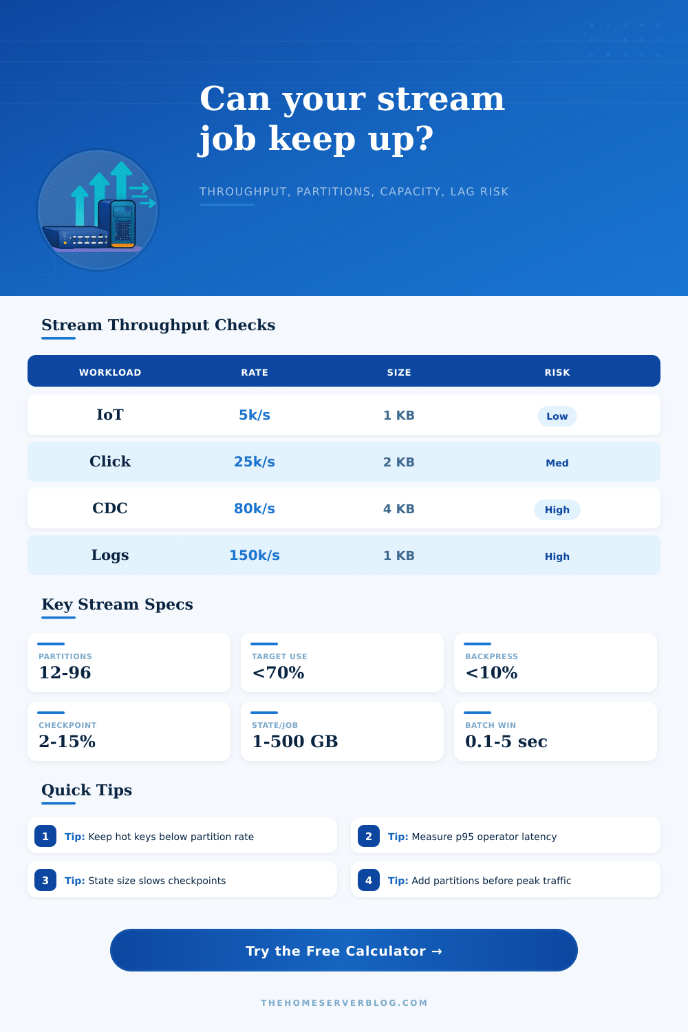
The page has some handy reference tables outlining common “healthy” operating thresholds. It suggests you leave yourself headroom for maintenance windows and bursts by keeping utilization below seventy percent.
Let me just say: Real world networks don’t follow a formula; they’re inherently chaotic, and no calculator can account to this. Some serialization libraries are more efficient than others. Each sink connector has its rate limit. Somewhere in your application logic, there may be an invisible N+1 query that only reveals itself at scale. This is what testing in staging is for.
The throughput math always apply though. There is X amount of I/O and CPU available to you per second. Each millisecond you spend on checkpointing or managing state is a millisecond you don’t get to move data through.
So, how do we scale stream processing? We scale it not by throwing hardware at the problem, but by recognizing the physics of data flow: control your partitioning strategy, control the amount of state managed, and monitor latency in each stage. Plug these specifics into the calculator above. Let it do the math for you to remove the guesswork from conversions and coefficients. Discover your breaking point without hitting it; then add a buffer.
For when the traffic spikes, you’ll be glad you planned for the silence that arrives after the lag begins.