Switch Oversubscription Calculator
Estimate access-to-uplink ratios, active host demand, burst pressure, east-west relief, and failover headroom for a home lab, office rack, Wi-Fi aggregation, or small server switch.
Switch oversubscription results
| Raw ratio | Typical fit | Watch for | Planning note |
|---|---|---|---|
| 1:1 to 2:1 | Storage, virtualization, spine-leaf | Host NIC bottlenecks | Good for iSCSI, NFS, vMotion, backups, and dense east-west traffic. |
| 2:1 to 4:1 | General home lab and office edge | Backup windows | Often balanced when only part of the edge is active at line rate. |
| 4:1 to 8:1 | Client access and Wi-Fi aggregation | Many simultaneous downloads | Usable when traffic is bursty and uplinks stay below target utilization. |
| 8:1 plus | IoT, cameras, low duty cycle clients | Unexpected east-to-north bursts | Needs clear traffic assumptions and monitoring after deployment. |
| Redundancy mode | Usable link rule | Failover behavior | Best use |
|---|---|---|---|
| No reserved uplink | All uplinks count | Capacity drops after a failure | Small labs, noncritical benches, temporary links. |
| N+1 reserved capacity | One uplink held back | One failure keeps planned capacity intact | Core uplinks, IDFs, and home office switches. |
| Active / standby pair | Half the links count | Standby takes over after failure | Simple firewall or router pairs without MLAG. |
| Dual-active MLAG | All links count, 95% factor | Peer loss reduces available path count | Dual-switch leaves, NAS, server access, resilient racks. |
| Stack or chassis uplinks | All links count, 90% factor | Member loss may rebalance paths | Stacked access switches with distributed uplinks. |
| Uplink speed | Common access pair | Approx edge fit | Practical note |
|---|---|---|---|
| 1G | 8 to 16 ports at 1G | 8:1 to 16:1 | Fine for light client switches, but easy to saturate with NAS copies. |
| 10G | 24 to 48 ports at 1G | 2.4:1 to 4.8:1 | Common home lab core uplink speed with good used-switch support. |
| 25G | 16 to 32 ports at 2.5G or 10G | 1.6:1 to 6.4:1 | Useful for Wi-Fi 6E, Wi-Fi 7, NAS, and compact server racks. |
| 40G | 48 ports at 1G or 10G | 1.2:1 to 12:1 | Good aggregate capacity, often via QSFP+ DAC or fiber modules. |
| 100G | 10G and 25G leaves | Low to moderate | Used when a home lab behaves like a small data center leaf. |
| Traffic profile | Active host percent | Average utilization | Burst factor |
|---|---|---|---|
| Home clients | 20% to 45% | 5% to 20% | 1.2x to 2.0x |
| Wi-Fi AP aggregation | 35% to 70% | 10% to 35% | 1.5x to 3.0x |
| Camera and IoT | 70% to 100% | 2% to 12% | 1.0x to 1.4x |
| Virtualization cluster | 50% to 100% | 25% to 70% | 1.5x to 4.0x |
| Backup or replication | 30% to 80% | 40% to 90% | 2.0x to 5.0x |
So you begin with a functioning network, then some jackass backsup four terabytes of photos at 2 AM. The switch stays online, but latency spikes. The game lags, and your Zoom call drops out.
Welcome to oversubscription in the wild, where your network barely keepss up… or snaps.
Why Your Network Switch Can Feel Slow
Home lab builders tend to focus on port count alone: they purchase a switch with twenty-four gigabit ports, and figure that means it will deliver twenty-four gigabits of network performance. That’s wrong; those twenty-four gigabits of potential is shared among the uplinks you have set up.
The calculator above does that math for you, translating unclear port counts into hard capacity limits. It forces you to face the realities of your setup well before bottleneck rears its head.
It’s an interesting problem with a simple underlying math that masks a bunch of complexity. There are two sets of ports: uplinks that face your storage or router and access ports that face your devices. How many uplinks versus how many access ports makes all the difference in terms of how much traffic can leave switch.
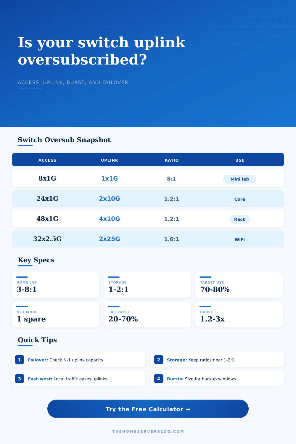
There are twenty-four gigabit ports against a single gigabit uplink. The ratio is twenty-four to one. Sounds terrible. And will be if every device try to talk at the same time. But that never happens.
Networks aren’t perfectly saturated most of the time. The challenge is guessing how many actual devices are talking at any given moment. In reality, most clients is idle while a few go out and download stuff and others stream something.
This is where active host percentage comes into play as an adjustable parameter. Get this right and tool begins to model real world behavior. Get it wrong and you either overbuy unnecessary bandwidth (too high guess) or end up suffering the lag spike you’re hoping to prevent (too low).
• There are also the bursts: Your backup job doesn’t give a damn about your nicely set average utilization; neither does your software update nor your virtual machine migration. These hammer the wire, so when we multiply your normal load with a burst factor of two, then suddenly our average load becomes twice as big, at least for some time. A double hit on an uplink that’s already close to its limit result in queueing delay.
So what’s the tool doing? It will compare your burst demand against the headroom you have on your uplinks. It’s a paper-based stress test.
And guess what: Where does the traffic go? If most of it remains local, if it flows from one workstation to another server sitting on the same switch, it will never touch the uplink. That eases the burden on exit door, that east-west traffic. The tool takes that into account and rewards designs that keeps data local, adjusting your effective load to match.
It all changes when you look at redundancy. Two uplinks seem to offer double the capacity…if both links are active simultaneously. But what about an active/standby pair? Now one of those links is sitting idle waiting for the other to fail. So your usable capacity drop by half.
You can also choose the redundancy mode from the calculator (stack, MLAG or N plus one). Each choice makes a unique mathematical difference to your available bandwidth. People often overlook this. They purchase dual uplinks because they want redundant connections, but then neglect to account for their capacity reduction in the event of a failover. The page includes a handy reference table that explains this. It shows exactly how various modes will impact your usable link count.
When it comes to storage traffic, you have to think differently. Close to one to one is good; the lower the better. Storage traffic doesn’t like sharing bandwidth (it’s jitter-sensitive), so if you’re running NFS or iSCSI, you’ll want this number closer to one to one. Even though the average may look fine, your storage traffic will feel slow with a high ratio.
Because office work and web browsing traffic tends to be short-lived and bursty, it can tolerate a higher ratio. The tool allows you to set a target ratio that makes sense for your use case. It won’t let you apply consumer-grade assumptions about the traffic to a database server, nor will it let you apply server-grade standards to a guest Wi-Fi network.
Planning a network is about managing expectations as much as wiring cables. Part of the process is managing expectations; connecting cables means making tradeoffs, and there’s no such thing as unlimited bandwidth at any price.
What do you want out of this: consistent low-latency for lots of light users, or raw throughput for a handful of heavy users? The calculator doesn’t answer that question for you. But it reveals the consequences. It tells you the gap between your port density and your eventual exit strategy.
When you see that, then you can determine whether that distance is tolerable to you. Maybe you’ll add an additional uplink. Or maybe you’ll reduce your estimate of the number of hosts you expect to run. Whatever you choose, it will be done by design, not by hoping for the best.
You should of known that. The real test of a good design isn’t what happens when things are quiet, but when they’re busy. You must know the boundaries and operate within them comfortabley. That’s what a network gets you.