HomeServerBlog Wi-Fi planning tool
Wi-Fi Channel Width Throughput Calculator
Estimate advertised PHY, practical goodput, per-client share, and channel-width tradeoffs from band, Wi-Fi generation, MCS, spatial streams, guard interval, airtime efficiency, interference, and regulatory availability.
1Wi-Fi presets
2Channel and radio inputs
Formula breakdown
Channel verdict
3Channel-width comparison grid
4Live planning metrics
Modulation and coding after generation clamp.
Band-specific usability factor.
Regulatory and channel-plan planning factor.
Goodput divided by estimated PHY.
5Wi-Fi reference tables
| MCS | Modulation | Coding | Typical need |
|---|---|---|---|
| MCS 0-2 | BPSK / QPSK | 1/2 to 3/4 | Robust edge coverage, low SNR, IoT, or long range. |
| MCS 3-7 | 16-QAM / 64-QAM | 1/2 to 5/6 | Normal Wi-Fi 4/5 baseline with moderate signal quality. |
| MCS 8-9 | 256-QAM | 3/4 to 5/6 | Clean 5 GHz or 6 GHz links with good SNR and low retries. |
| MCS 10-11 | 1024-QAM | 3/4 to 5/6 | Wi-Fi 6 and 6E peak client links near the AP. |
| MCS 12-13 | 4096-QAM | 3/4 to 5/6 | Wi-Fi 7 peak rates with excellent signal and clean 6 GHz spectrum. |
| Generation | Max MCS here | Wide-channel note | Planning behavior |
|---|---|---|---|
| Wi-Fi 4 / 802.11n | MCS 7 per stream | 20 or 40 MHz | Use 20 MHz on 2.4 GHz unless the band is very quiet. |
| Wi-Fi 5 / 802.11ac | MCS 9 | 80 or 160 MHz | 80 MHz is the common home-lab sweet spot on 5 GHz. |
| Wi-Fi 6 / 6E / 802.11ax | MCS 11 | 80 or 160 MHz | OFDMA and better aggregation help dense homes and offices. |
| Wi-Fi 7 / 802.11be | MCS 13 | 160 or 320 MHz | 320 MHz is mainly a 6 GHz clean-spectrum plan. |
| Width | Best fit | Common tradeoff | HomeServerBlog use case |
|---|---|---|---|
| 20 MHz | 2.4 GHz, crowded 5 GHz, IoT | Lower peak speed, strongest coexistence. | IoT VLANs, old clients, apartment networks. |
| 40 MHz | 5 GHz mixed networks | Moderate throughput with less neighbor overlap. | Outdoor mesh, garage APs, cameras. |
| 80 MHz | Most 5 GHz homes | Good balance of speed and channel reuse. | Laptops, phones, NAS sync, office Wi-Fi. |
| 160 MHz | Clean 5 GHz DFS or 6 GHz | Higher peak speed with fewer usable channels. | VR, workstations, wireless backhaul. |
| 320 MHz | Wi-Fi 7 on 6 GHz | Huge peak rate but tight channel availability. | Same-room Wi-Fi 7 and MLO planning. |
| Regulatory plan | Typical availability | Watch item | Calculator meaning |
|---|---|---|---|
| 2.4 GHz 20 MHz | 100% | Only three non-overlapping 20 MHz channels in many regions. | Good for availability, not for peak throughput. |
| 5 GHz non-DFS | 55% | Fewer contiguous 80/160 MHz choices. | Conservative plan when DFS events are not acceptable. |
| 5 GHz with DFS | 75% | Radar detection can force channel changes. | Better capacity if devices and location tolerate DFS. |
| 6 GHz low power indoor | 90% | Indoor-only client and AP rules may apply. | Best everyday place for 160 MHz channels. |
| 6 GHz standard power | 80% | AFC rules and local availability can limit operation. | Outdoor or higher-power 6 GHz planning factor. |
6Wi-Fi channel-width tips
You buy a gigabit-capable router, then run a speed test from your desk, only to see it return a fraction of that rate. One says this; the other says that. That doesn’t have to be about your internet plan. Much of the time, it’s Wi-Fi’s invisible math: the logic of channels.
Enter your settings into calculator up top (band, generation, interference) and let it do the math for you. No more guesswork on why your throughput feels so sluggish, even with a clean link.
Why Your Wi-Fi Is Slow
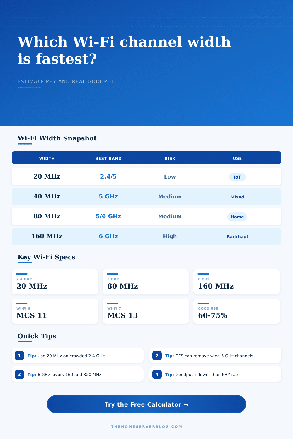
That’s the trade-off at the heart of Wi-Fi planning: wider channels means faster speeds, but also greater exposure to congestion. A wide channel is like a big funnel, if the radio spectrum around you are crowded, then it will catch all kinds of noise from the neighborhood. Narrower channels can be quieter. Sure, they might not go as fast, but they slice right through interference.
What’s important here is knowing which matter more for your space. Do you want maximum burst download speed, or do you care about consistent reliability (like for dozens of IoT device pinging around in the background)?
First up: Look at what band you’re using. In the case of 2.4 GHz band, this is a shared resource. Your neighbor’s network, your baby monitor, everyone’s microwave… They is all fighting for some space. On the 2.4 GHz band, keeping your channel width at 20 MHz is almost always the right move. It limits how fast you can go, but it preserves your connection in a noisy environment. Forcing 40 MHz onto 2.4 GHz are typically a recipe for frustration. Your actual goodput plummets, retries spike and signal-to-noise ratio goes down.
With the 5 GHz and 6 GHz bands, there’s more breathing room. That means you can play around with wider channels such as 80 MHz (and potentially up to 160 MHz). Regulatory availability is the catch. Not all of available channels in these bands are created equal. Some are dynamic frequency selection channels, which mean your access point has to listen for radar signals before jumping on the channel. When it does pick up one, it will kick you off immediately. The result is intermittent drops that make it seem like your connection sucks.
The tool accounts for this regulatory availability factor by reminding you that having a theoretically wide channel doesn’t do you any good if you’re unable to remain on it long enough to use it.
The modulation and coding scheme is another hidden killer. Even if you have a Wi-Fi 6 router with high MCS rates supported, it’s limited by the rate your client device can achieve. While a new phone may reach MCS 11 or higher, an older laptop might only be able to get up to MCS 9. Similarly, spatial streams is important. No matter how wide the channel, a two stream connection will always lose out to four.
The calculator lets you see this trade-off in action. It displays the difference between physical layer rate (theoretical maximum) and the goodput (what you actualy use once overhead has been removed). This is the key point: Goodput is reality; PHY rate is marketing. Acknowledgments, frame headers, and retransmissions eats bandwidth. These losses are minor in a perfect vacuum. Add them all up in a real-world environment of competing networks, metal appliances, and drywall.
Model this loss using the airtime efficiency input. You are assuming 90 percent efficiency in a crowded apartment. You’re lying to yourself. More realisticly, maybe it’s only 60 percent.
Don’t chase the biggest number. You’ll get fewer bytes through a wide channel continually retrying its packets then a narrow one sending clean frames. You should of want consistency. Match what your environment allows with your hardware abilities using the reference tables as your guide. Go wide if you have a back haul link between two points with a clear line of sight. Go narrow and add access points if you’re covering a dense office full of clients. The math will point you to the right balance, understanding the space points you to the inputs.