Wi-Fi Spatial Stream Calculator
Plan realistic Wi-Fi throughput from AP stream count, client NSS, MIMO mode, channel width, MCS, guard interval, MU-MIMO group size, antenna chains, SNR quality, and airtime efficiency.
Spatial stream throughput plan
This planner estimates throughput from common PHY relationships and practical efficiency factors. Real AP firmware, chipset support, channel utilization, DFS events, antenna orientation, client drivers, and traffic direction can shift measured results.
| Device class | Typical streams | What caps it | Planning note |
|---|---|---|---|
| IoT sensor or camera | 1x1 | Client radio | Use low stream count and conservative MCS for edge coverage. |
| Phone or tablet | 1x1 to 2x2 | Client antennas | Most mobile devices will not use more than two streams. |
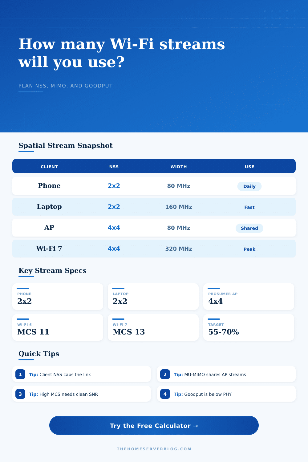
| Mainstream laptop | 2x2 | Client Wi-Fi card | Best modeled as two streams with 80 or 160 MHz if SNR is clean. |
| High-end client bridge | 3x3 to 4x4 | Both endpoints | Useful for fixed wireless bridges and same-room high throughput links. |
| MIMO mode | Stream allocation | Best fit | Calculator behavior |
|---|---|---|---|
| Single-user MIMO | One client at a time | One fast laptop or phone | Scheduled NSS equals the negotiated AP/client/chain minimum. |
| SU with beamforming | One client, cleaner link | Same-room or stable rooms | Adds a small link-quality factor before payload efficiency. |
| Downlink MU-MIMO | AP streams split across clients | Several compatible clients downloading | Aggregate NSS can rise toward the AP stream ceiling. |
| Uplink MU / OFDMA | Clients share uplink rounds | Dense rooms and mixed uploads | Uses scheduler efficiency and MU group size in the model. |
| Wi-Fi 7 multi-link style | Multiple links may coordinate | Wi-Fi 7 clients near APs | Applies a modest coordination gain for planning only. |
| SNR class | MCS ceiling | Delivery factor | Typical observation |
|---|---|---|---|
| Edge / unstable | MCS 4 | 72% | Coverage edge, retries, roaming, or weak 2.4 GHz clients. |
| Fair room-to-room | MCS 7 | 82% | Usable signal with walls, neighbors, or moderate interference. |
| Good home SNR | MCS 9 | 90% | Typical clean 5 GHz home-lab client close to the AP. |
| Excellent same-room | MCS 11 | 96% | Strong signal, low retries, and stable high-rate modulation. |
| Lab-clean | MCS 13 | 99% | Best-case Wi-Fi 7 style planning with very clean spectrum. |
| Width | Stream impact | Common tradeoff | Home lab use |
|---|---|---|---|
| 20 MHz | Lowest per-stream PHY | Best coexistence and range behavior. | IoT, 2.4 GHz, garage, and crowded apartments. |
| 40 MHz | About double 20 MHz | Moderate speed with easier channel reuse. | Outdoor links, mixed 5 GHz, camera networks. |
| 80 MHz | Common 5 GHz baseline | Good balance of speed and spectrum reuse. | Laptops, phones, NAS sync, normal home APs. |
| 160 MHz | High per-stream PHY | Needs cleaner 5 GHz DFS or 6 GHz spectrum. | VR, workstation links, and wireless backhaul. |
| 320 MHz | Wi-Fi 7 peak width | Very spectrum-hungry and best on 6 GHz. | Same-room Wi-Fi 7 and lab testing. |
Your friend buys an eight-antenna Wi-Fi 7 router and expects to edit video wirelessly. He plugs his laptop in, runs a speedtest, and gets same numbers he had last year. It’s not typicaly the router’s fault. The problem is usualy spatial streams.
Wi-Fi have these parallel data lanes called spatial streams that carry information. Most folks assume that more antennas means faster speed. Not true. While more antennas might help reception, they is limited by number of simultaneous streams your device supports.
Why More Antennas Do Not Mean Faster Wi-Fi
Two streams? Your laptop probably does that. Two streams? Your phone probably does that too. Your access point might have four or eight stream. It’s not going to force-feed more streams to your devices than they can take and the weak-link in the chain almost always becomes the bottleneck.
Once you input what your environment is and which device you have, the calculator do all the math for you. Input client capability, the AP capability, and let the tool tell you what effective number is. Usually that will be the lowest of those numbers.
This is part most folks don’t understand. They think about the ceiling of their hardware, rather than negotiated reality.
What is pipe size? While that’s important (a 160 MHz channel has twice the capacity of an 80 MHz one), it isn’t as big an issue as you’d imagine. Doubling the channel width doesn’t do anything if link drops down to lower modulation schemes because of poor signal-to-noise ratio. That’s where the SNR class input comes into play.
If you’ve got a clean signal in same room, you can goes with high-order modulations like 1024-QAM or even 4096-QAM. If signal’s being fought through two drywall partitions, you might be stuck at basic QPSK. The throughput difference is huge. Depending on what SNR you select, the tool will clamp max modulation index so you don’t plan on getting a lab result in noisy apartment.
Airtime matters, too. Wi-Fi is a half-duplex medium. On any given channel, only one device may speak at a time. Every handshake, acknowledgement and request has to be sent through the router which manages them all. That overhead consume a huge chunk of your theoretical maximum.
Most planners plan that you’ll get 80% of PHY rate. But in busy home, you might only get 60% or even less. You can tweak this efficiency factor in calculator. With a dozen active devices sharing the air, goodput per client drop dramatically. And it doesn’t matter how many spatial streams the AP provides. It’s still shared resource, not a dedicated wire.
With MU-MIMO things get interesting again because it enable the AP to talk with multiple clients at once. But it doesn’t adds any bandwidth. It slices what’s already there. Say you’ve got 4×4 AP. And you’ve got two client that are both 2×2. Well, then the AP can send two streams to each one of them in parallel. Latency per client go down. Aggregate throughput may be same. But if you want to run a voice call or play a game, lower latency (not necessarily higher absolute speeds) make a big difference.
Consistency is key. You’ll see the tradeoffs laid out in reference tables on the page. Why a high-throughput AP isn’t the same than a high density one? One handles volume, the other handles concurrency. In practice, you’ll probably end up with some sort of middle-ground between those two extremes. Balance speed, density, and coverage.
When you see your numbers, consider not only the aggregate PHY rate (a marketing figure) or even total usable goodput (an engineering figure). Consider also the per-client share. Because that’s what your users will see.
Firstly: Who are your heavy users? Is it one machine that does big file transfers? Focus on SNR and stream count for that one. Are they gamers and streamers? Focus on airtime efficiency and multiple-user scheduling.
Where do you think your particular configuration falls apart? How can you see that with this tool? It makes real-world expectations out of ideas about radio. Instead of wondering if the wall’s thick or new router is slow, you simply know what the limit is. Knowing the limit should of enabled you to plan effectively.