WiFi MU-MIMO Throughput Calculator
Estimate usable 802.11ac, 802.11ax, or 802.11be MU-MIMO throughput from channel width, MCS, spatial streams, client stream mix, airtime efficiency, contention, retries, and scheduled client groups.
MU-MIMO throughput estimate
PHY values are planning estimates for one AP radio. Real drivers may limit MU client count, disable MU for some traffic classes, or fall back to SU-MIMO when a client mix cannot be grouped efficiently.
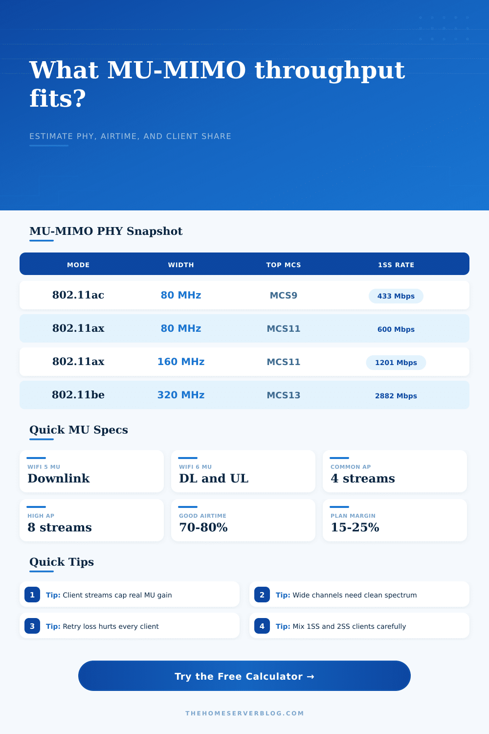
| PHY generation | Top MCS used | 80 MHz 1SS | 160 MHz 1SS | 320 MHz 1SS |
|---|---|---|---|---|
| 802.11ac VHT | MCS 9, 256-QAM 5/6 | 433 Mbps | 867 Mbps | Not defined |
| 802.11ax HE | MCS 11, 1024-QAM 5/6 | 600 Mbps | 1201 Mbps | Not defined |
| 802.11be EHT | MCS 13, 4096-QAM 5/6 | 721 Mbps | 1441 Mbps | 2882 Mbps |
| Planning note | Calculator scales lower MCS | Uses GI factor | Caps by standard | Single radio only |
| Channel width | Best fit | MU-MIMO impact | Planning caution |
|---|---|---|---|
| 20 MHz | 2.4 GHz or dense 5 GHz | Lower PHY but more channel reuse | Often better for many low-rate clients |
| 40 MHz | Moderate homes | Doubles 20 MHz PHY under clean CCA | Can collide with neighbors on 2.4 GHz |
| 80 MHz | Common Wi-Fi 5/6 high throughput | Good balance for 2SS laptops | DFS and co-channel load still matter |
| 160 MHz | 6E or clean 5 GHz labs | High PHY for 2SS and 4SS clients | Retry rate can erase the gain |
| 320 MHz | Wi-Fi 7 6 GHz | Very high EHT PHY ceiling | Only available on compatible APs/clients |
| Client stream type | Typical devices | Grouping effect | Throughput note |
|---|---|---|---|
| 1-stream | Phones, IoT, small tablets | Needs more clients to fill AP streams | Great for MU fairness, weak for peak rate |
| 2-stream | Laptops, phones, handheld consoles | Fills 4x4 AP with two active clients | Most common real-world planning case |
| 3-stream | Older premium laptops, adapters | May waste one stream on 4x4 grouping | Driver support varies by chipset |
| 4-stream | Workstations, bridges, backhaul nodes | Can consume a full 4x4 group alone | Often better tested as SU or backhaul |
| Scenario | AP and clients | Good assumption | Risk to model |
|---|---|---|---|
| Home office laptops | 4x4 AP, 4 to 8 mostly 2SS clients | 80 MHz, MCS 9-11, 65-75% airtime | Printers and IoT may not join MU groups |
| Apartment evening load | 4x4 AP, many 1SS/2SS clients | 40 or 80 MHz, 20-40% contention loss | CCA backoff can dominate PHY gains |
| 6E file sync | 4x4 AP, 2SS laptops, clean 6 GHz | 160 MHz, MCS 11, low retry loss | Distance can drop MCS quickly |
| Wi-Fi 7 workstation area | 4x4 or 8x8 AP, 2SS/4SS clients | 160-320 MHz, EHT MCS 12-13 | One-radio estimate excludes MLO aggregation |
Are you getting Gigabit speeds? Are there four streams? Are you getting full bars? But your laptop gets half of that. If it’s lucky, on a good day. Your video buffers while the router sits there saying “all good.” What gives?
Wireless is a shared resource, negotiated among all devices at any instant in real time. Throughput isn’t a pipe; it isn’t even a pipe with constant size. It’s a dynamic thing that needs math. Our calculator does this for you after you input conditions and your mix of client. You don’t have to guess how much of your bandwidth survives antenna-to-application.
Why Your Wi-Fi Is Slower Than It Says
Here’s where multi-user MIMO shakes things up: The access point can speak with multiple devices in parallel. Clients don’t have to take turns. They’re given simultaneous transmissions. Sounds like free speed? Sure, if you put together the right group. A four-stream access point won’t provide four times the speed to just a single phone. It requires multiple clients. Or a very capable client that will fill out its spatial streams. Put together a bunch of one-stream phones and their total rate remains unchanged, but each phone gets a fairer slice of airtime. And sometimes fairness is worth more then raw peak speed.
So why do the inputs? Because inputs are a reflection off the real world. The ceiling depends on channel width. And channel width depends on whether or not the spectrum is clean. Yes, you can choose one hundred and sixty megahertz channels on paper. But if your neighbor is broadcasting on that exact same frequency, your device spends most of its time waiting for the channel to clear. You don’t see the contention loss. It will continue until it hurt. And that’s where the tool comes into play. It lets you adjust for neighbor activity. This is typically the largest variable in apartment living. Co-channel interference eats up twenty to forty percent of your theoretical capacity before you send your first packet. That’s how dense building work.
There’s another wrinkle: modulation and coding scheme (MCS). Using a higher index MCS enables you to send more data on each symbol, but it also means that if signal quality drops by even a little bit, your device will need to back off down to a lower MCS. And that’s a constant thing as you wander from room to room. Add in retries, and this compounds the issue. Each time a packet gets retried, that’s all overhead. It burns up airtime without bringing any actual data home. Throw in scheduling frames, acknowledgements and MAC headers, and even in ideal conditions, the actual fraction of airtime being used for efficiently getting data around can be less than eighty percent. The calculator takes those losses into account to get you a usable number, not a marketing number.
Where folks tend to get hung up is stream diversity. Sure, you may have an awesome four-by-four access point. Yet, it’s surrounded by all these other cheap smart bulbs and other legacy IoT sensor that just have one antenna. So they can’t use the additional streams. That means wasted capacity. Throw in some phones with one stream and some laptops with two streams, and the balance is off and now the scheduler has to work around that. On the page there’s a reference table that shows how much airtime various types of client will fill in the air. The idea is to make sure your access point matches what you actually have in your home. Plan ahead to create a buffer.
Networks don’t run at a constant load. Backups begin, updates download, and you’re flooded. A buffer of 10-20% provides room for that peak usage without crashing your network. But more importantly, there is room for the slow decay caused by physical barriers and distance. Signals bounce off metal objects; walls absorb them. It all adds noise. This therefore requires strong settings instead of aggressive ones.
There are Wi-Fi 7, 6, and 5 versions. When choosing Wi-Fi radios, don’t just look at the generation name alone. Wi-Fi 7 adds higher modulation and wider channels, which only pays off if you have compatible clients. If you upgrade your access point without upgrading any of the devices attached to it, you gain little. The bottleneck shifts to the endpoint. You need to understand this dynamic when making investment decisions. Invest in the technology that matches your weakest link. Which may or may not be the most expensive radio.
Consistency is the final test of any networking solution. It doesn’t matter if your net gets gigabits one minute and dialup the next. It’s not about peaks; it’s about stability. And there’s no better way to estimate that stability prior to hardware purchase than with these tables and tools. They force you to face the realities of protocol overhead, device capability, and interference.
Airtime tax isn’t something you can just ignore. But when you do take it into account, you can create an actual working network, which is where we started with this question, how much speed do I really get? The answer is that it is always less than advertised, and now you know exactly why.